Estimating Negative Variance

A few weeks ago, my post-doc adviser, Mandy, asked me to examine a scenario. It was a basic random effects model of the form

\[ W_{ijk} = X_{ik} + E_{ijk}, \quad i = 1,\ldots,n, \quad j = 1,\ldots,J, \quad k = 1,\ldots,K, \]

in which the response for subject \(i\) for replicate \(j\) and component \(k\) (\(W_{ijk}\)) is generated through a latent effect (\(X_{ik}\)) and some observational noise (\(E_{ijk}\)). The model can be applied to neuroimaging in which different unobserved structures or networks have some effect on blood oxygen levels. The main goal is to estimate the variance of the latent effect, and for ease of convention, independent normal random variable distributions are assumed on both the latent effect and the observation noise. That is,

\[ X_{ik} \overset{i.i.d.}{\sim} \text{Normal}\left(\mu_k, \tau_k^2\right), \quad E_{ijk} \overset{i.i.d.}{\sim} \text{Normal}(0,\sigma^2).\]

The following function can be used to generate data from this model:

latent_random_effects_data <- function(n,J,K, mu, tau2, sigma2) {
  E <- array(rnorm(n*J*K, sd = sqrt(sigma2)), dim = c(n,J,K))
  X <- sapply(seq(K), function(k) {
    X_k <- rnorm(n, mean = mu[k], sd = sqrt(tau2[k]))
    return(X_k)
  })
  means <- X %o% array(1,dim = J)
  W <- aperm(means,perm = c(1,3,2)) + E
  return(W)
}

Mandy told me that there was trouble estimating the latent effect variance (\(\tau_k^2\)) in this model because sometimes the estimates would come back negative, which is impossible. I decided to code this up for myself to see, and maybe apply some Bayesian method to fix (see my previous post). The latent effect variance is estimated through the use of basic variance probability calculations, considered in a simple case when the number of replicates (\(J\)) is just 2:

\[\begin{align*} \text{Var}(W_{ijk}) & = \text{Var}(X_{ik} + E_{ijk}) \\ & = \text{Var}(X_{ik}) + \text{Var}(E_{ijk}) \\ W_{i1k} - W_{i2k} & = (X_{ik} + E_{i1k}) - (X_{ik} - E_{i2k}) \\ \text{Var}(W_{i1k} - W_{i2k}) & = 2\text{Var}(X_{ik}) + 2\text{Var}(E_{i1k}) \\ \text{Var}(X_{ik}) & = \text{Var}(W_{ijk}) - \text{Var}(E_{ijk}) \end{align*}\]

So how does this end up working out on the generated data model? This will be tested in a scenario with 100 subjects, 2 replicates, and 5 components. The true averages for the components will be \(\boldsymbol{\mu} = (\mu_1,\mu_2,\mu_3,\mu_4,\mu_5) = (2,4,6,8,10)\), the component variances will be set to \(\boldsymbol{\tau}^2 = (\tau_1^2,\tau_2^2,\tau_3^2,\tau_4^2,\tau_5^2) = (1,2,3,4,5)\), and the observation noise variance will be set to \(\sigma^2 = 5\). A boxplot for the data within the components can be seen below.

set.seed(47403) # The seed is the zip code for Indiana University
W <-
  latent_random_effects_data(
    n = 100,
    J = 2,
    K = 5,
    mu = seq(2,10,length.out = 5),
    tau2 = 1:5,
    sigma2 = 5
  )

boxplot(apply(W,3,identity), xlab = "Component", ylab = "Observed Data",
        main = "Data summaries within the different components")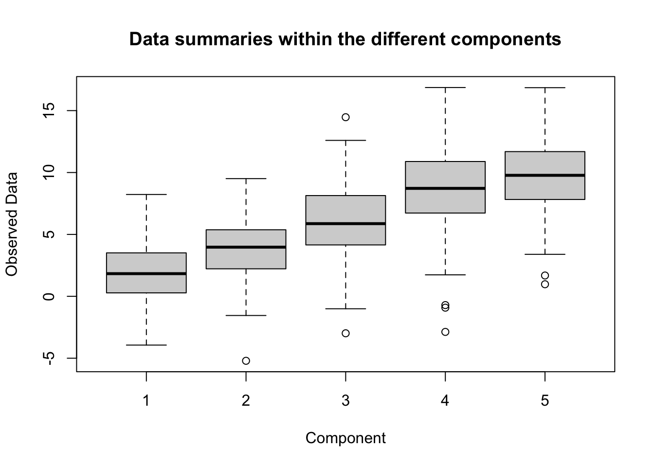

The following steps are followed to estimate the variance of the latent components: 1) Find the variance for each replicate-component pair (rep_component_var) 2) Find the replicate variance by averaging the replicate-component variances across components (rep_var) 3) Estimate the noise variance by estimating the variance of the differences between replicates (visit_diff) and finding the variances of the differences across components (noise_var) 4) Estimate the latent variances by taking the differences between the replicate variances and the noise variances

The above steps are carried out in R below:

rep_component_var <- apply(W,2:3,var)
rep_var <- apply(rep_component_var,2,mean)
visit_diff <- W[,1,] - W[,2,]
noise_var <- apply(visit_diff,2,var) / 2
latent_var <- rep_var - noise_var
latent_var

## [1] -0.103987  0.709116  3.491612  4.451649  3.212830

The problem is visible in the first component’s variance estimate, which happens to be negative. The true values from the data generation are (1, 2, 3, 4, 5), and the components with higher variances are indeed positive (and somewhat close to their true values). This is something of a paradox: The variance of the sum of two random variables is somehow less than the sum of the individual variances within the first component. One possible solution to this problem is to estimate the component variances using Bayesian estimates, which was outlined using MCMC for a single component in a previous post. This can be generalized to any number of components for comparison, using the posterior mode to estimate the component variances.

source("basic_bayesian_random_effects.R")
latent_effects_mcmc_results <- latent_random_effects_mcmc(
  W, 
  variance_priors = "eb_IG", # Using empirical Bayes inverse gamma priors on the variances
  hyperparameters = list(prior_means = apply(W,3,mean)) # Using empirical values for mu_k
  )

## Starting MCMC
## MCMC finished, 10000 samples in 11.504 seconds

For the sake of thoroughness, it’s a good idea to at least examine the trace plots for the latent variances to see if the MCMC converges. As a note, the first 500 samples from the posterior distribution were discarded as a burn-in, even though the initial values were set using the empirical estimates of all parameter values.

library(ggplot2)
tau2_df <- reshape2::melt(latent_effects_mcmc_results$tau2, 
                          varnames = c("Component","Posterior Draw"), 
                          value.name = "Variance")
tau2_df$Component <- paste("Component",tau2_df$Component)
ggplot(tau2_df) + 
  geom_line(aes(x = `Posterior Draw`, y = `Variance`)) + 
  facet_grid(Component~., scales = "free")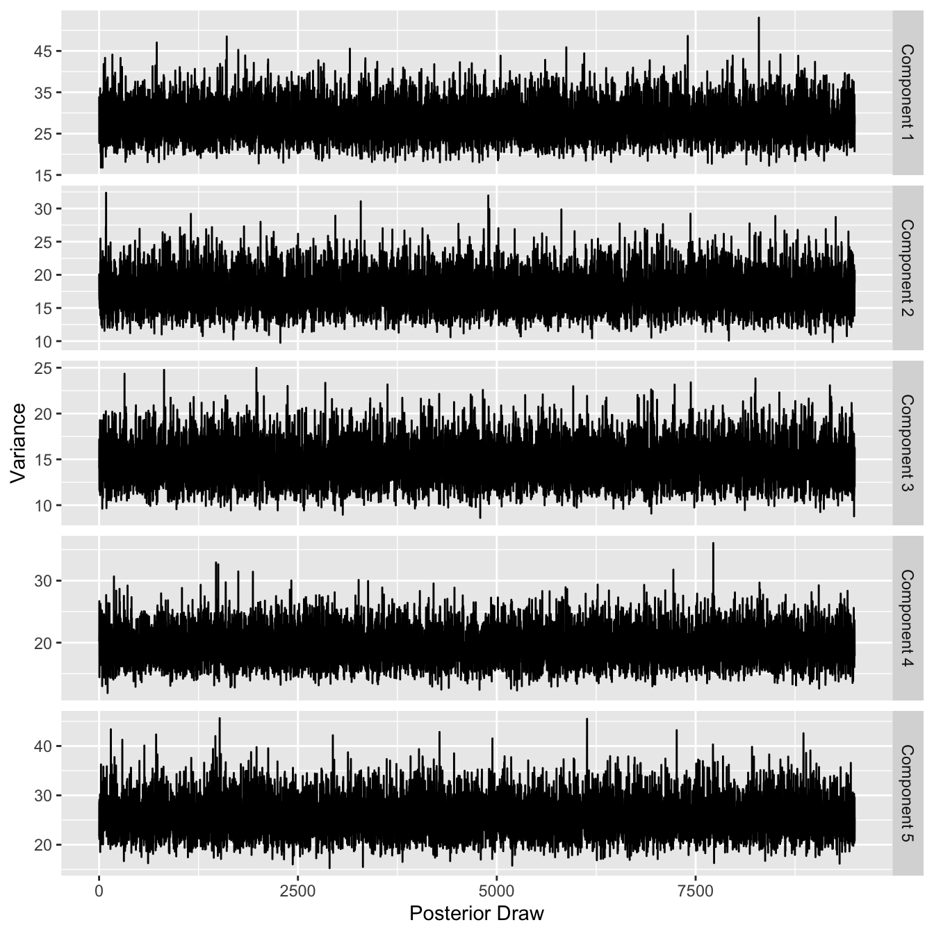

These plots look to show values that are consistently in the same area for the posterior draws, which is a good indicator for convergence of the MCMC. Estimating the variances using the modes of the marginal posterior distributions is done below:

latent_variance_densities <- apply(latent_effects_mcmc_results$tau2,1,density)
Bayes_latent_var <- sapply(latent_variance_densities, function(vd_k) {
  return(vd_k$x[which.max(vd_k$y)])
})
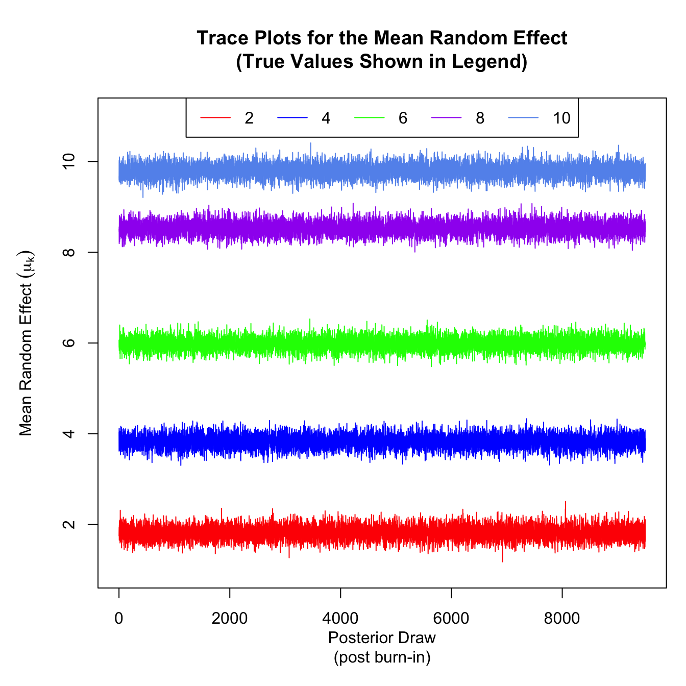
Bayes_latent_var

## [1] 27.61533 16.40985 14.10919 18.24378 25.31000

There is a good and a bad takeaway here. The good news is that there are no negative variance estimates here, but the bad news is that the estimates are not near the true values. This is interesting, as the means for the latent effects (\(\mu_k: \, k = 1,2,3,4,5\)) are all very well-estimated, as is the noise variance. Plots for these parameters can be seen at the bottom, for the curious. It is interesting to note that the two basic estimation methods (Bayesian and frequentist) have such a distinct tradeoff, which opens up questions about modifications to those methods to get the best of both worlds.

par(mar = c(5,5,5,1))
plot(latent_effects_mcmc_results$sigma2, type = 'l', 
     xlab = "Posterior Draw\n(post burn-in)",
     ylab = expression(paste("Noise Variance ",(sigma^2))),
     main = "Trace Plot for Observation Variance\n(True Value is 5)")
abline(h = 5, col = 'white', lty = 3)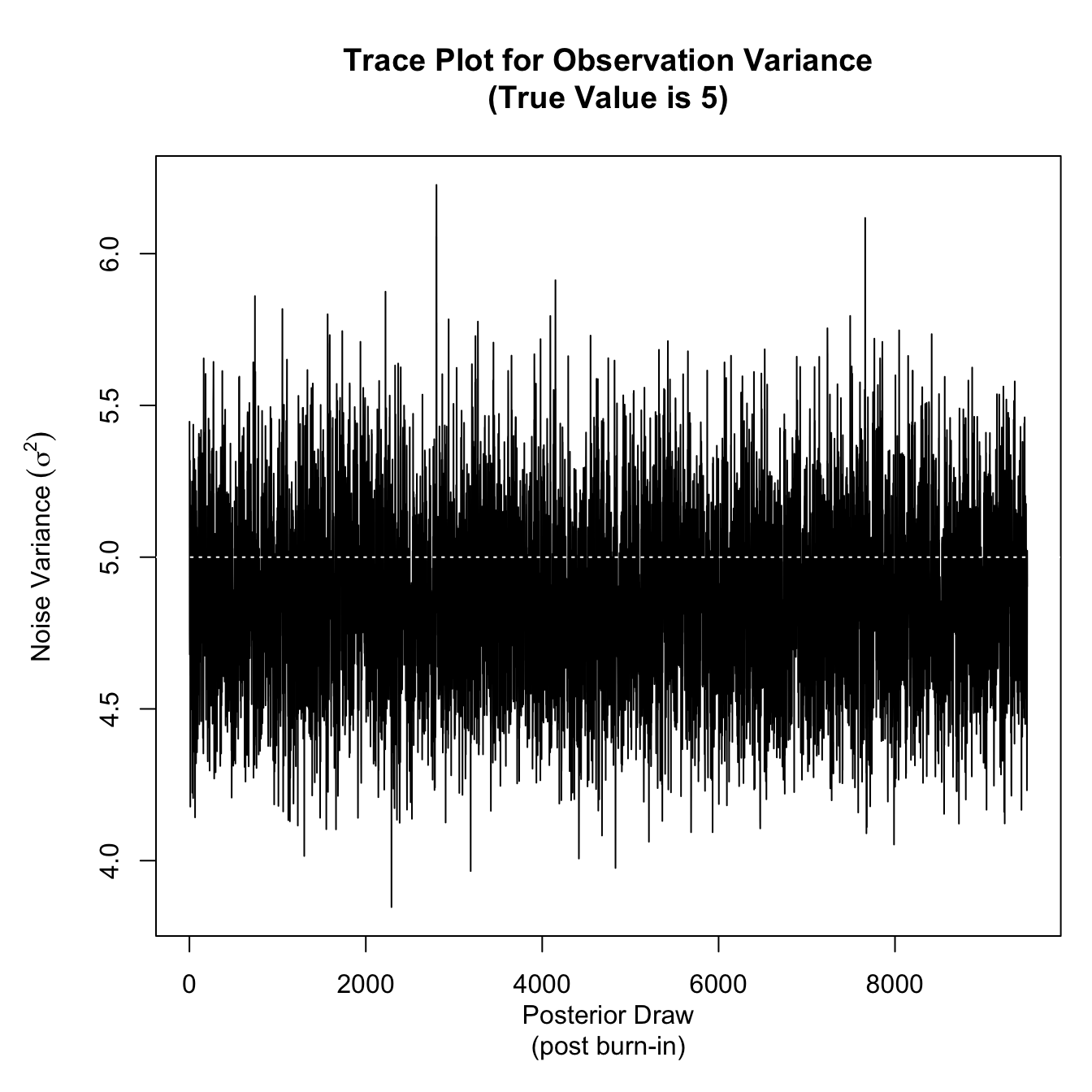

trace_mean_effect <- apply(latent_effects_mcmc_results$X,2:3,mean)
plot(x = as.numeric(summary(seq(ncol(trace_mean_effect)))),
     y = as.numeric(summary(c(trace_mean_effect))),
     ylim = c(1,11),
     type = 'n', xlab = "Posterior Draw\n(post burn-in)", 
     ylab = expression(paste("Mean Random Effect ",(mu[k]))),
     main = "Trace Plots for the Mean Random Effect\n(True Values Shown in Legend)")
lines(trace_mean_effect[1,], col = 'red')
lines(trace_mean_effect[2,], col = 'blue')
lines(trace_mean_effect[3,], col = 'green')
lines(trace_mean_effect[4,], col = 'purple')
lines(trace_mean_effect[5,], col = 'cornflowerblue')
legend("top", lty = 1, legend = seq(2,10,length.out = 5), col = c('red','blue','green','purple','cornflowerblue'), horiz = T)