Bayesian Random Effects Models

Consider a scenario in which noisy data are observed, with variance driven by two primary sources: signal and noise. We can write the data generation as

\[ W_{ij} = X_i + E_{ij}, \quad i = 1,\ldots, n, \quad j = 1,2 \]

Here, consider \(X_i\) as the signal and \(E_{ij}\) as the noise, with values generated from zero-mean normal distributions.

\[ X_i \sim \text{Normal}(0,\sigma_x^2), \quad E_{ij} \sim \text{Normal}(0,\sigma_e^2) \]

set.seed(47403) # Set this so the results are always the same
sigma2_e_true <- 3
sigma2_x_true <- 5
n <- 100
E <- matrix(rnorm(n*2, sd = sqrt(sigma2_e_true)),n,2)
X <- rnorm(n,sd = sqrt(sigma2_x_true))
W <- cbind(X,X) + E

If we want to solve for the variance parameters \(\sigma_x^2\) and \(\sigma_e^2\), as Bayesians we could give each parameter a prior and look at the posterior distributions of both. For convenience, give both parameters a relatively uninformative inverse gamma prior (for conjugacy).

\[ \sigma_x^2, \sigma_e^2 \overset{iid}{\sim} \text{Inverse Gamma} (0.1, 1)\] Now that we have the full model, we can find that the posterior full-conditional distributions are relatively easy to come across:

\[X_i | W_{i\cdot},\sigma_e^2, \sigma_x^2 \sim \text{Normal}\left( \left( \frac{2}{\sigma_x^2} + \frac{1}{\sigma_e^2} \right)^{-1} \frac{\sum_{j=1}^2 W_{ij}}{\sigma_e^2}, \left( \frac{2}{\sigma_x^2} + \frac{1}{\sigma_e^2} \right)^{-1} \right),\]

\[\sigma_x^2 | X_{\cdot} \sim \text{Inverse Gamma} \left( \frac{n}{2} + 0.1, 1 + \frac{1}{2}\sum_{i=1}^{n} X_i^2 \right),\]

\[\sigma_e^2 | X_\cdot, W_{\cdot\cdot} \sim \text{Inverse Gamma}\left( n + 0.1, 1 + \frac{1}{2} \sum_{i = 1}^n \sum_{j = 1}^2 (W_{ij} - X_i)^2 \right).\]

Without doing much more work, we can sample from the posterior distribution using MCMC and make some inference! So how does it do?

# W is the observed data and S is the number of samples to draw from the 
# posterior distribution.
mcmc_function <- function(W, S = 10000, a_sigma_e = 0.1, b_sigma_e = 1, 
                          a_sigma_x = 0.1, b_sigma_x = 1, B = 100) {
  # Start with initial conditions
  sigma2_e <- mean(apply(W,1,var))
  sigma2_x <- var(apply(W,1,mean))
  X <- apply(W,1,mean)
  
  # Preallocate storage for draws from the posterior distribution
  mcmc_results <- list(
    X = matrix(NA,n,S),
    sigma2_e = numeric(S),
    sigma2_x = numeric(S)
  )
  
  # Run the MCMC for 10k iterations
  start_time <- proc.time()[3]
  for(s in seq(S)) {
    X <- rnorm(n, (1 / (1/sigma2_e + 2/sigma2_x)) * apply(W,1,sum)/sigma2_e, 
               sd = sqrt((1 / (1/sigma2_e + 2/sigma2_x))))
    sigma2_x <- 1/rgamma(1,n/2 + a_sigma_x, b_sigma_x + sum(X^2)/2)
    sigma2_e <- 1/rgamma(1,n + a_sigma_e, b_sigma_e + sum(apply(W,2,`-`,y =X)^2)/2)
    mcmc_results$X[,s] <- X
    mcmc_results$sigma2_e[s] <- sigma2_e
    mcmc_results$sigma2_x[s] <- sigma2_x
  }
  total_time <- proc.time()[3] - start_time
  cat("Total MCMC run time:",S,"draws in",total_time,"seconds \n")
  # Remove burn-in
  mcmc_results$X <- mcmc_results$X[,-seq(B)]
  mcmc_results$sigma2_e <- mcmc_results$sigma2_e[-seq(B)]
  mcmc_results$sigma2_x <- mcmc_results$sigma2_x[-seq(B)]
  return(mcmc_results)
}
mcmc_results <- mcmc_function(W)

## Total MCMC run time: 10000 draws in 2.076 seconds

It’s always a good idea to see how the draws from the posterior distribution vary over the draws that are made, as there can be a problem if there is too much dependence between one draw and the next. These types of plots are referred to as trace plots.

par(mfrow=c(2,1), mar = c(5,5,1,1))
plot(mcmc_results$sigma2_e, type='l', main = "", ylab = expression(sigma[e]^2), xlab = "Iteration")
plot(mcmc_results$sigma2_x, type='l', main = "", ylab = expression(sigma[x]^2), xlab = "Iteration")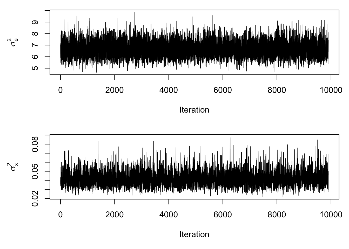

These plots look good, as the values for the parameters very quickly adhere around a horizontal line without a strong discernable trend. We can look at the density plots for the posterior draws of \(\sigma_x^2\) and \(\sigma_e^2\) and see how close they were to the true values:

par(mfrow=c(1,2))
plot(density(mcmc_results$sigma2_e), main = "", xlab = expression(sigma[e]^2))
abline(v = sigma2_e_true, col = 'red')
plot(density(mcmc_results$sigma2_x), main = "", xlab = expression(sigma[x]^2))
abline(v = sigma2_x_true, col = 'red')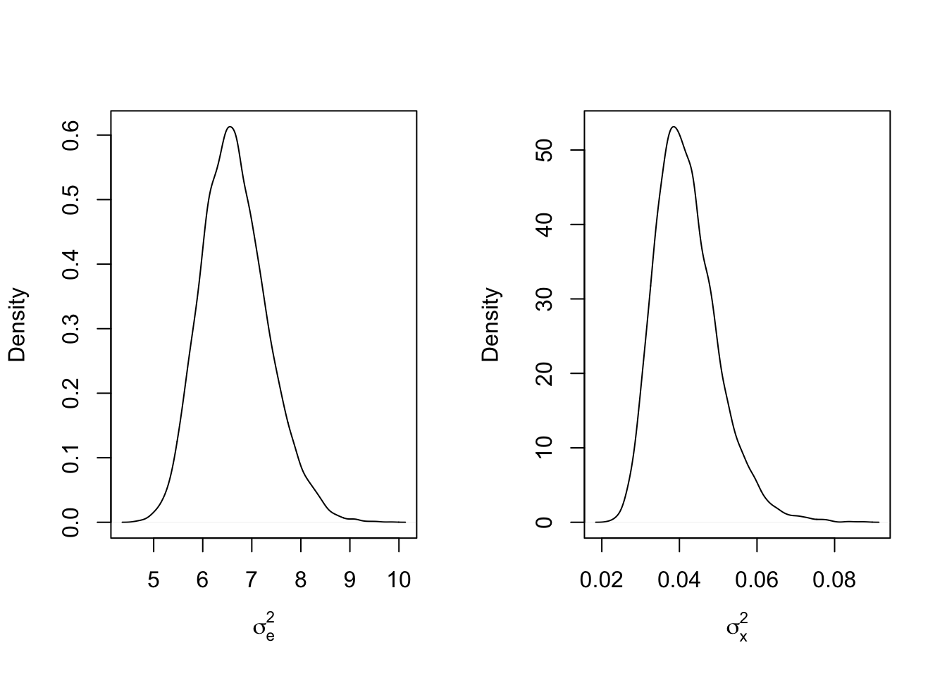

What happened here? It looks almost like the posterior draws for the two variance parameters bounced closer to the values of the opposite parameter! This is a problem know as identifiability, in which two values are being summed or multiplied to account for the same effect. In this case, both \(\sigma_x^2\) and \(\sigma_e^2\) are used to account for variance in \(\mathbf{W}\). What happens if \(\sigma_x^2 = 100\) and \(\sigma_e^2 = 1\)?

set.seed(47403) # Set this so the results are always the same
sigma2_e_true <- 1
sigma2_x_true <- 100
n <- 100
E <- matrix(rnorm(n*2, sd = sqrt(sigma2_e_true)),n,2)
X <- rnorm(n,sd = sqrt(sigma2_x_true))
W <- cbind(X,X) + E

mcmc_results2 <- mcmc_function(W)

## Total MCMC run time: 10000 draws in 2.079 seconds

par(mfrow=c(1,2))
plot(density(mcmc_results2$sigma2_e), main = "", xlab = expression(sigma[e]^2))
abline(v = sigma2_e_true, col = 'red')
plot(density(mcmc_results2$sigma2_x), main = "", xlab = expression(sigma[x]^2))
abline(v = sigma2_x_true, col = 'red')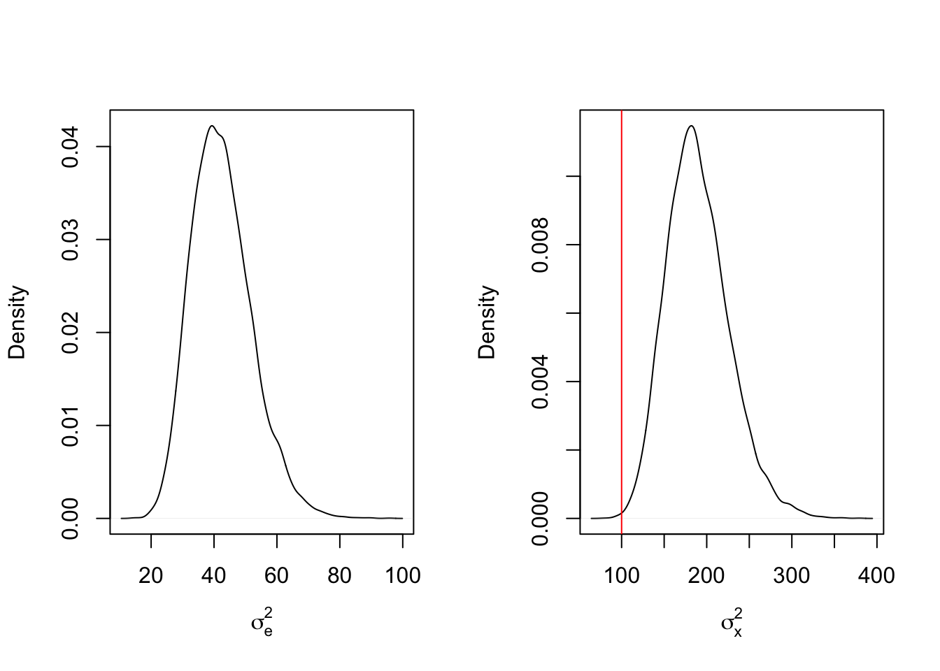

We see from these results that the difference bouys the posterior draws for \(\sigma_x^2\) upward, to the point that most of the marginal posterior density is higher than the true value. This increase in variance leads to high draws for \(X_i\), resulting in higher draws for \(\sigma_e^2\). What happens when the sample size is increased from 100 to 1,000?

set.seed(47403) # Set this so the results are always the same
sigma2_e_true <- 1
sigma2_x_true <- 100
n <- 1000
E <- matrix(rnorm(n*2, sd = sqrt(sigma2_e_true)),n,2)
X <- rnorm(n,sd = sqrt(sigma2_x_true))
W <- cbind(X,X) + E

mcmc_results3 <- mcmc_function(W)

## Total MCMC run time: 10000 draws in 14.356 seconds

par(mfrow=c(1,2))
plot(density(mcmc_results3$sigma2_e), main = "", xlab = expression(sigma[e]^2))
abline(v = sigma2_e_true, col = 'red')
plot(density(mcmc_results3$sigma2_x), main = "", xlab = expression(sigma[x]^2))
abline(v = sigma2_x_true, col = 'red')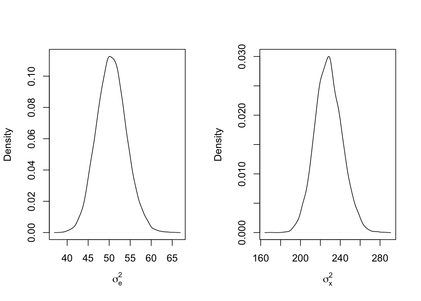

While there is less skew in the marginal posterior distributions, the inflation of the variance parameters has only gotten worse! A Bayesian might wonder if the priors may be playing a part in this strange switching. After all, the mean of an inverse gamma distribution with shape 0.1 and rate 1 is technically infinite. What if the priors were more informative, say with means around 1 and 100 for \(\sigma_e^2\) and \(\sigma_x^2\), respectively?

set.seed(47403) # Set this so the results are always the same
sigma2_e_true <- 1
sigma2_x_true <- 100
n <- 100
E <- matrix(rnorm(n*2, sd = sqrt(sigma2_e_true)),n,2)
X <- rnorm(n,sd = sqrt(sigma2_x_true))
W <- cbind(X,X) + E

mcmc_results4 <- mcmc_function(W, a_sigma_e = 2, b_sigma_e = 2, a_sigma_x = 2, b_sigma_x = 200)

## Total MCMC run time: 10000 draws in 2.05 seconds

par(mfrow=c(1,2))
plot(density(mcmc_results4$sigma2_e), main = "", xlab = expression(sigma[e]^2))
abline(v = sigma2_e_true, col = 'red')
plot(density(mcmc_results4$sigma2_x), main = "", xlab = expression(sigma[x]^2))
abline(v = sigma2_x_true, col = 'red')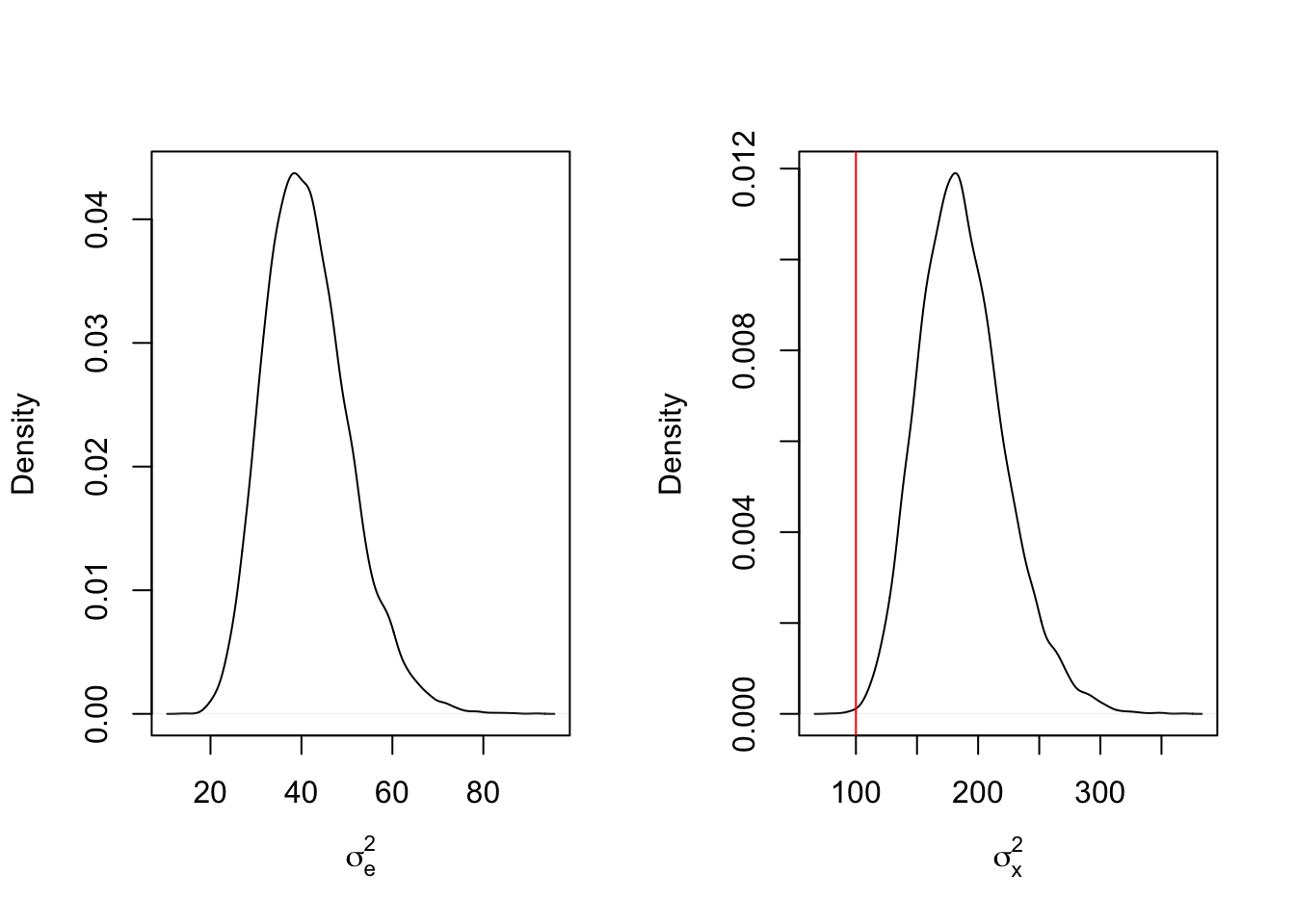

This shows that the influence of the prior distributions appears to be negligible. What does increasing the sample size back to 1000 have in this case?

set.seed(47403) # Set this so the results are always the same
sigma2_e_true <- 1
sigma2_x_true <- 100
n <- 1000
E <- matrix(rnorm(n*2, sd = sqrt(sigma2_e_true)),n,2)
X <- rnorm(n,sd = sqrt(sigma2_x_true))
W <- cbind(X,X) + E

mcmc_results5 <- mcmc_function(W, a_sigma_e = 2, b_sigma_e = 2, a_sigma_x = 2, b_sigma_x = 200)

## Total MCMC run time: 10000 draws in 14.304 seconds

par(mfrow=c(1,2))
plot(density(mcmc_results5$sigma2_e), main = "", xlab = expression(sigma[e]^2))
abline(v = sigma2_e_true, col = 'red')
plot(density(mcmc_results5$sigma2_x), main = "", xlab = expression(sigma[x]^2))
abline(v = sigma2_x_true, col = 'red')

Since the data now plays a stronger role, the priors have even less of an effect, variance inflation is stronger here. What if the parameters themselves are switched? That is, what if the observation variance \(\sigma_e^2\) and the effect variance \(\sigma_x^2\) are set such that the effect variance is smaller than the observation variance?

set.seed(47403) # Set this so the results are always the same
sigma2_e_true <- 100
sigma2_x_true <- 1
n <- 100
E <- matrix(rnorm(n*2, sd = sqrt(sigma2_e_true)),n,2)
X <- rnorm(n,sd = sqrt(sigma2_x_true))
W <- cbind(X,X) + E

mcmc_results6 <- mcmc_function(W, a_sigma_e = 2, b_sigma_e = 200, a_sigma_x = 2, b_sigma_x = 2)

## Total MCMC run time: 10000 draws in 2.039 seconds

par(mfrow=c(1,2))
plot(density(mcmc_results6$sigma2_e), main = "", xlab = expression(sigma[e]^2))
abline(v = sigma2_e_true, col = 'red')
plot(density(mcmc_results6$sigma2_x), main = "", xlab = expression(sigma[x]^2))
abline(v = sigma2_x_true, col = 'red')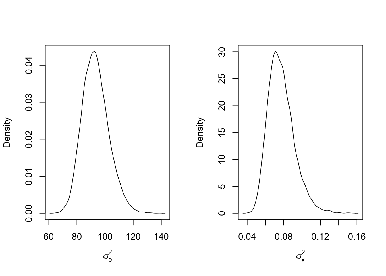

Now we can see that the posterior inference is reflective of the true values, though the variance for the random effect is dramatically shrunken towards zero. What does this mean? In cases where there are random effects with mean 0, the largest source of variance gets pooled into the observation variance while the smaller variance is reserved for the random effect variance. Another test may shed some light here. What if the mean of the random effect is sufficiently large relative to the observation variance, say 50?

set.seed(47403) # Set this so the results are always the same
sigma2_e_true <- 100
sigma2_x_true <- 1
n <- 100
E <- matrix(rnorm(n*2, sd = sqrt(sigma2_e_true)),n,2)
X <- rnorm(n,mean = 50, sd = sqrt(sigma2_x_true))
W <- cbind(X,X) + E

mcmc_results7 <- mcmc_function(W, a_sigma_e = 2, b_sigma_e = 200, a_sigma_x = 2, b_sigma_x = 2)

## Total MCMC run time: 10000 draws in 2.009 seconds

par(mfrow=c(1,2))
plot(density(mcmc_results7$sigma2_e), main = "", xlab = expression(sigma[e]^2))
abline(v = sigma2_e_true, col = 'red')
plot(density(mcmc_results7$sigma2_x), main = "", xlab = expression(sigma[x]^2))
abline(v = sigma2_x_true, col = 'red')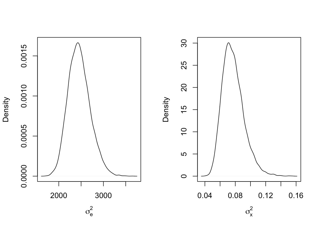

There has been almost no change in the posterior distribution of \(\sigma_x^2\). but the estimate for \(\sigma_e^2\) is huge! Clearly there is something happening here that is

set.seed(47403) # Set this so the results are always the same
sigma2_e_true <- 100
sigma2_x_true <- 1
n <- 100
E <- matrix(rnorm(n*2, sd = sqrt(sigma2_e_true)),n,2)
X <- rnorm(n,mean = 1000, sd = sqrt(sigma2_x_true))
W <- cbind(X,X) + E

mcmc_results8 <- mcmc_function(W, a_sigma_e = 2, b_sigma_e = 200, a_sigma_x = 2, b_sigma_x = 2)

## Total MCMC run time: 10000 draws in 2.033 seconds

par(mfrow=c(1,2))
plot(density(mcmc_results8$sigma2_e), main = "", xlab = expression(sigma[e]^2))
abline(v = sigma2_e_true, col = 'red')
plot(density(mcmc_results8$sigma2_x), main = "", xlab = expression(sigma[x]^2))
abline(v = sigma2_x_true, col = 'red')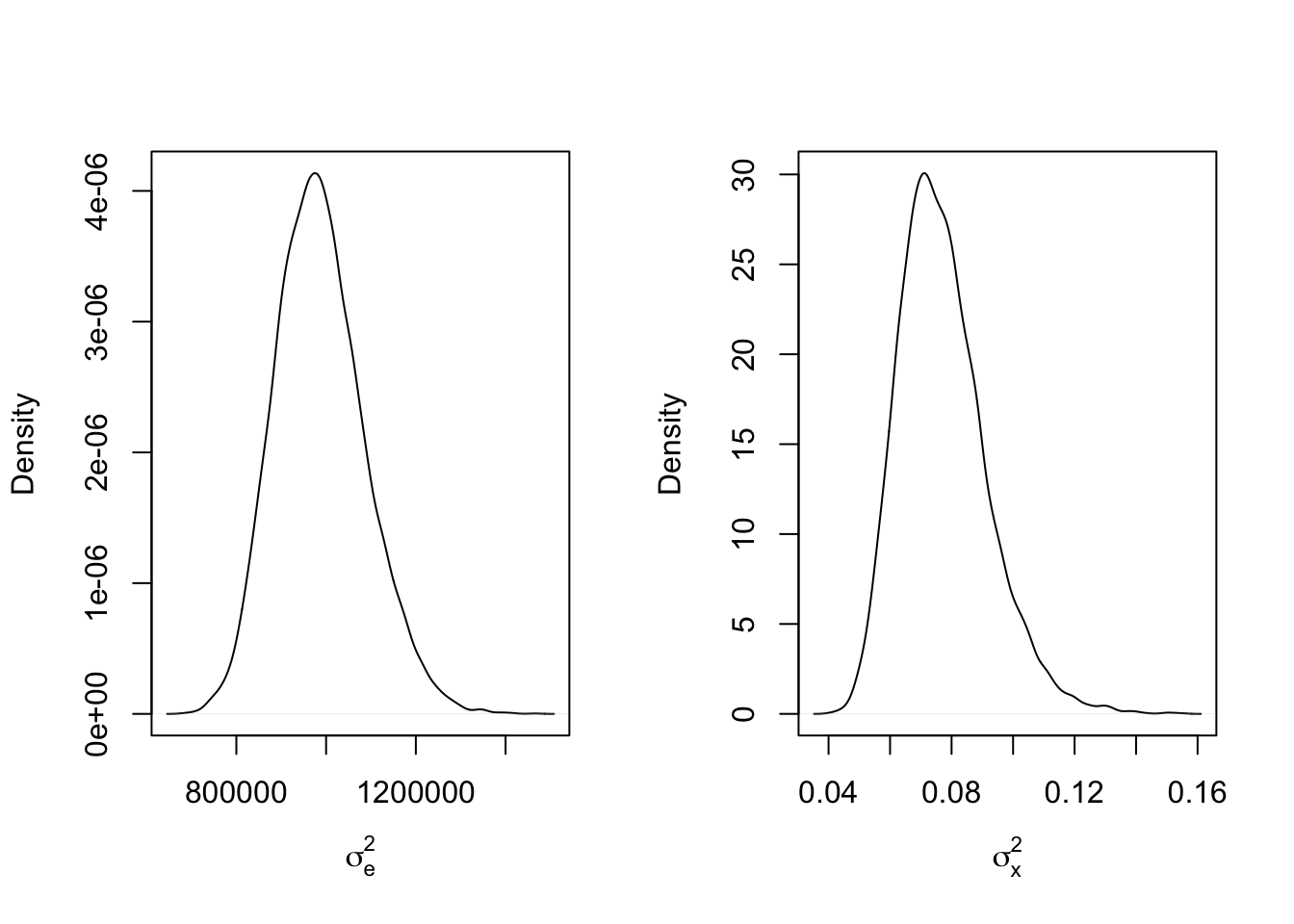

This is certainly something to keep in mind when designing your models and especially when attempting to model variance using Bayesian methods!