Word Clouds

Last summer, I was fortunate to be able to take a two-day short course with Abel Rodriguez here at UCSC. He based the course on the quarter-long Art of Data Visualization course that he had taught that winter quarter. It was super interesting, and it motivated me to try a few things on my own, including a word cloud. I use Google Voice, which saves all of my text messages in spreadsheet format. I downloaded the information that I needed, and I set off.

I decided to make one for the text messages with my wife, and another one for a friend of mine that also took the short course with me. They came out as follows:

##### Word cloud fun
library(XML)
library(tm)

## Loading required package: NLP

library(wordcloud)

## Loading required package: RColorBrewer

library(RColorBrewer)

Lisa’s word cloud

Lisa <- read.csv("~/Downloads/Lisa.csv") #Note: Replace with your own .csv
Lisa_df <- data.frame(doc_id = Lisa$timestamp, text = Lisa$message)
Lisa.corpus <- Corpus(DataframeSource(Lisa_df))
Lisa.corpus <- tm_map(Lisa.corpus, removePunctuation) # Take out punctuation
Lisa.corpus <- tm_map(Lisa.corpus, content_transformer(tolower)) # Make everything lower case
Lisa.corpus <- tm_map(Lisa.corpus, removeWords, stopwords("english")) # Get rid of common English words
Lisa.tdm <- TermDocumentMatrix(Lisa.corpus) # Get the words organized by the documents they appear in
Lisa.m <- as.matrix(Lisa.tdm)
Lisa.v <- sort(rowSums(Lisa.m),decreasing=TRUE) # Order the words by frequency
Lisa.d <- data.frame(word = names(Lisa.v),freq = Lisa.v) # Put it into a data frame including the words themselves
pal2 <- brewer.pal(8,"Dark2") # Define the color palette for the plot
wordcloud(Lisa.d$word,Lisa.d$freq,scale = c(8,.2),
          min.freq = 3,random.order = FALSE, rot.per = .15, colors = pal2)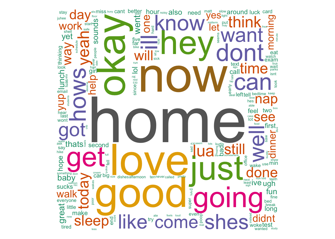

Kurtis’s word cloud

Kurtis <- read.csv("~/Downloads/Kurtis.csv") #Note: Replace with your own .csv
Kurtis_df <- data.frame(doc_id = Kurtis$timestamp, text = Kurtis$message)
Kurtis.corpus <- Corpus(DataframeSource(Kurtis_df))
Kurtis.corpus <- tm_map(Kurtis.corpus, removePunctuation) # Take out punctuation
Kurtis.corpus <- tm_map(Kurtis.corpus, content_transformer(tolower)) # Make everything lower case
Kurtis.corpus <- tm_map(Kurtis.corpus, removeWords, stopwords("english")) # Get rid of common English words
Kurtis.tdm <- TermDocumentMatrix(Kurtis.corpus) # Get the words organized by the documents they appear in
Kurtis.m <- as.matrix(Kurtis.tdm)
Kurtis.v <- sort(rowSums(Kurtis.m),decreasing=TRUE) # Order the words by frequency
Kurtis.d <- data.frame(word = names(Kurtis.v),freq = Kurtis.v) # Put it into a data frame including the words themselves
pal2 <- brewer.pal(8,"Dark2") # Define the color palette for the plot
wordcloud(Kurtis.d$word,Kurtis.d$freq,scale = c(8,.2),
          min.freq = 3,random.order = FALSE, rot.per = .15, colors = pal2)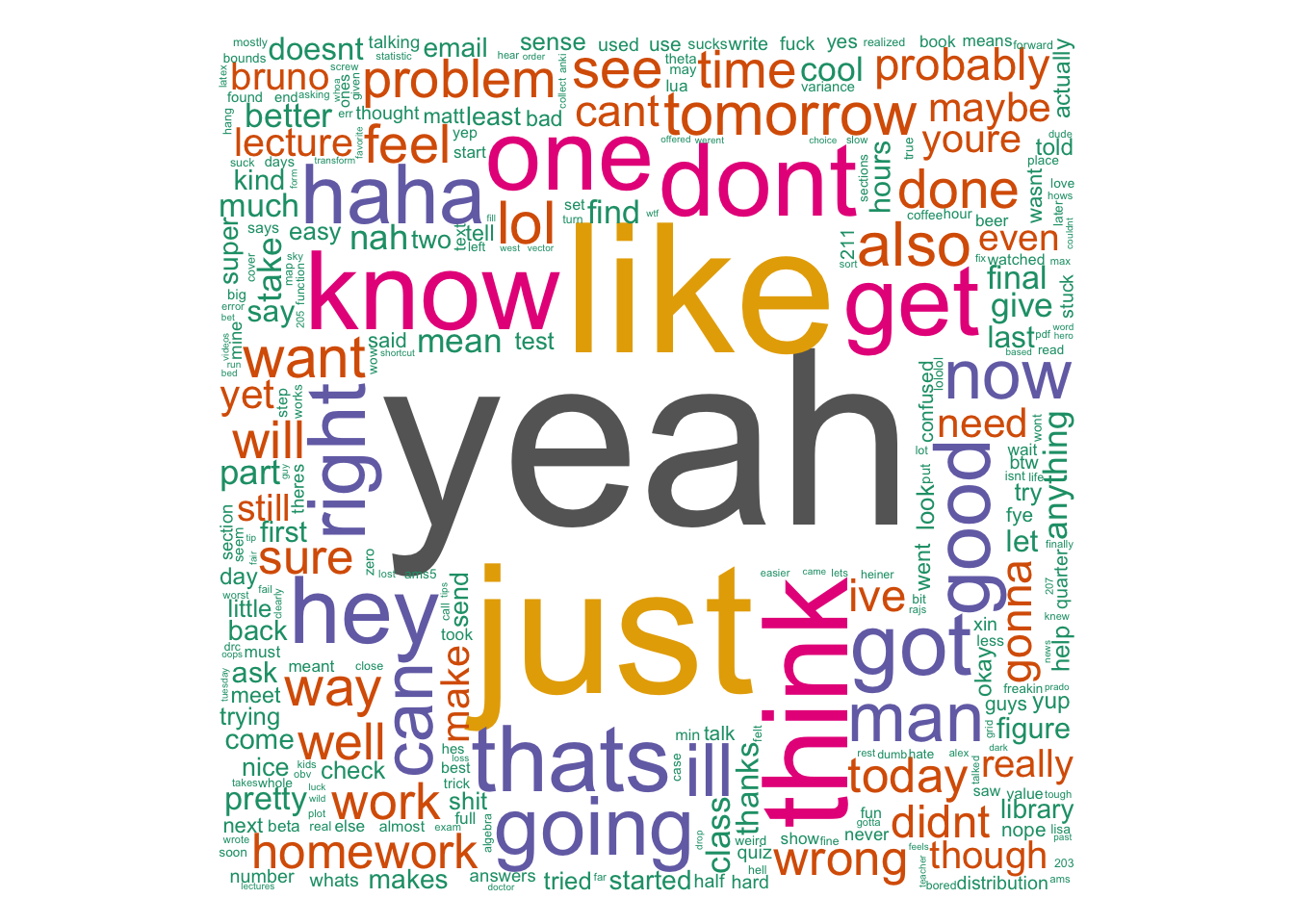

There’s a bit of a difference between the two, huh?